install.packages("devtools")
library(devtools)
install_github("timelyportfolio/d3treeR")Hands-on Exercise 5e: Treemap Visualisation with R
1 Overview
A Treemap displays hierarchical data as a set of nested rectangles. Each group is represented by a rectangle, whose area is proportional to its value. In this exercise, we will learn how to manipulate transaction data into a treemap structure by using selected functions provided in dplyr package. Then, we will learn how to plot static treemap by using treemap package. Finally, we will learn how to design an interactive treemap by using d3treeR package.
2 Getting Started
2.1 Installing and loading the packages
For this exercise, the following R packages will be used.
treemap is a space-filling visualization of hierarchical structures. This function offers great flexibility to draw treemaps.
treemapify draws the treemap without the help of the
ggplot2geoms, or for some edge cases such as creating interactive treemaps with ‘RShiny’.d3treeRis the primary function for creating interactive d3.js treemaps from various data types in R.
pacman::p_load(treemap, treemapify, d3treeR, tidyverse) 2.2 Data import
The data of private property transaction records in 2018 is extracted from REALIS portal of Urban Redevelopment Authority (URA).
realis2018 <- read_csv("data/realis2018.csv")2.3 Preparing the Data
The data frame realis2018 is in transaction record form, which is highly disaggregated and not appropriate to be used to plot a treemap. Hence, we will need perform the following steps to manipulate and prepare a data frame that is appropriate for treemap visualisation:
group transaction records by Project Name, Planning Region, Planning Area, Property Type and Type of Sale
compute Total Unit Sold, Total Area, Median Unit Price and Median Transacted Price by applying appropriate summary statistics on No. of Units, Area (sqm), Unit Price ($ psm) and Transacted Price ($) respectively.
We will use group_by() and summarize() of dplyr package.
group_by()breaks down a data frame into specified groups of rows. When you then apply the verbs above on the resulting object they’ll be automatically applied “by group”.
Grouping affects the verbs as follows:
grouped
select()is the same as ungroupedselect(), except that grouping variables are always retained.grouped
arrange()is the same as ungrouped; unless you set.by_group= TRUE, in which case it orders first by the grouping variables.mutate()andfilter()are most useful in conjunction with window functions (likerank(), ormin(x) == x). They are described in detail in vignette(“window-functions”).sample_n()andsample_frac()sample the specified number/fraction of rows in each group.summarise()computes the summary for each group.
Let us look at how to group summaries without pipe and with pipe (%>%) .
To learn more about pipe, visit this excellent article: Pipes in R Tutorial For Beginners.
realis2018_grouped <- group_by(realis2018, `Project Name`,
                               `Planning Region`, `Planning Area`,
                               `Property Type`, `Type of Sale`)
realis2018_summarised <- summarise(realis2018_grouped,
                          `Total Unit Sold` = sum(`No. of Units`, na.rm = TRUE),
                          `Total Area` = sum(`Area (sqm)`, na.rm = TRUE),
                          `Median Unit Price ($ psm)` = median(`Unit Price ($ psm)`, na.rm = TRUE),
                          `Median Transacted Price` = median(`Transacted Price ($)`, na.rm = TRUE))
Note
The argument na.rm = TRUE removes the missing values prior to computation.
This is a more efficient method.
realis2018_summarised <- realis2018 %>%
  group_by(`Project Name`,`Planning Region`,
           `Planning Area`, `Property Type`,
           `Type of Sale`) %>%
  summarise(`Total Unit Sold` = sum(`No. of Units`, na.rm = TRUE),
            `Total Area` = sum(`Area (sqm)`, na.rm = TRUE),
            `Median Unit Price ($ psm)` = median(`Unit Price ($ psm)`, na.rm = TRUE),
            `Median Transacted Price` = median(`Transacted Price ($)`, na.rm = TRUE))
3 Designing Static Treemaps with treemap Package
We will only explore the major arguments for designing elegent and yet truthful treemaps.
We shall plot a treemap showing the distribution of median unit prices and total unit sold of resale condominium by geographic hierarchy in 2018 by filtering the data frame first.
realis2018_selected <- realis2018_summarised %>%
filter(`Property Type` == "Condominium", `Type of Sale` == "Resale")The treemap is designed using three core arguments of treemap(), namely: index, vSize and vColor.
Show the code
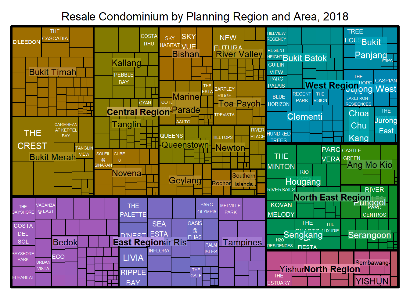
treemap(realis2018_selected,
        index=c("Planning Region", "Planning Area", "Project Name"),
        vSize="Total Unit Sold",
        vColor="Median Unit Price ($ psm)",
        title="Resale Condominium by Planning Region and Area, 2018",
        title.legend = "Median Unit Price (S$ per sq. m)"
        )
Note
index: The index vector must consist of at least two column names or else no hierarchy treemap will be plotted. If multiple column names are provided, the first name is the highest aggregation level, the second name the second highest aggregation level, and so on.vSize: The column must not contain negative values. This is because its vaues will be used to map the sizes of the rectangles of the treemaps.vColor: used in combination with the argumenttypeto determine the colours of the rectangles. Without definingtype,treemap()assumestype = index, in our case, the hierarchy of planning areas. Hence, the above treemap is wrongly coloured (we want to have different intensity colours for different median unit prices).
Set vColor and Type to make the colour work correctly.
Show the code
treemap(realis2018_selected,
        index=c("Planning Region", "Planning Area", "Project Name"),
        vSize="Total Unit Sold",
        vColor="Median Unit Price ($ psm)",
        type = "value",
        title="Resale Condominium by Planning Region and Area, 2018",
        title.legend = "Median Unit Price (S$ per sq. m)" )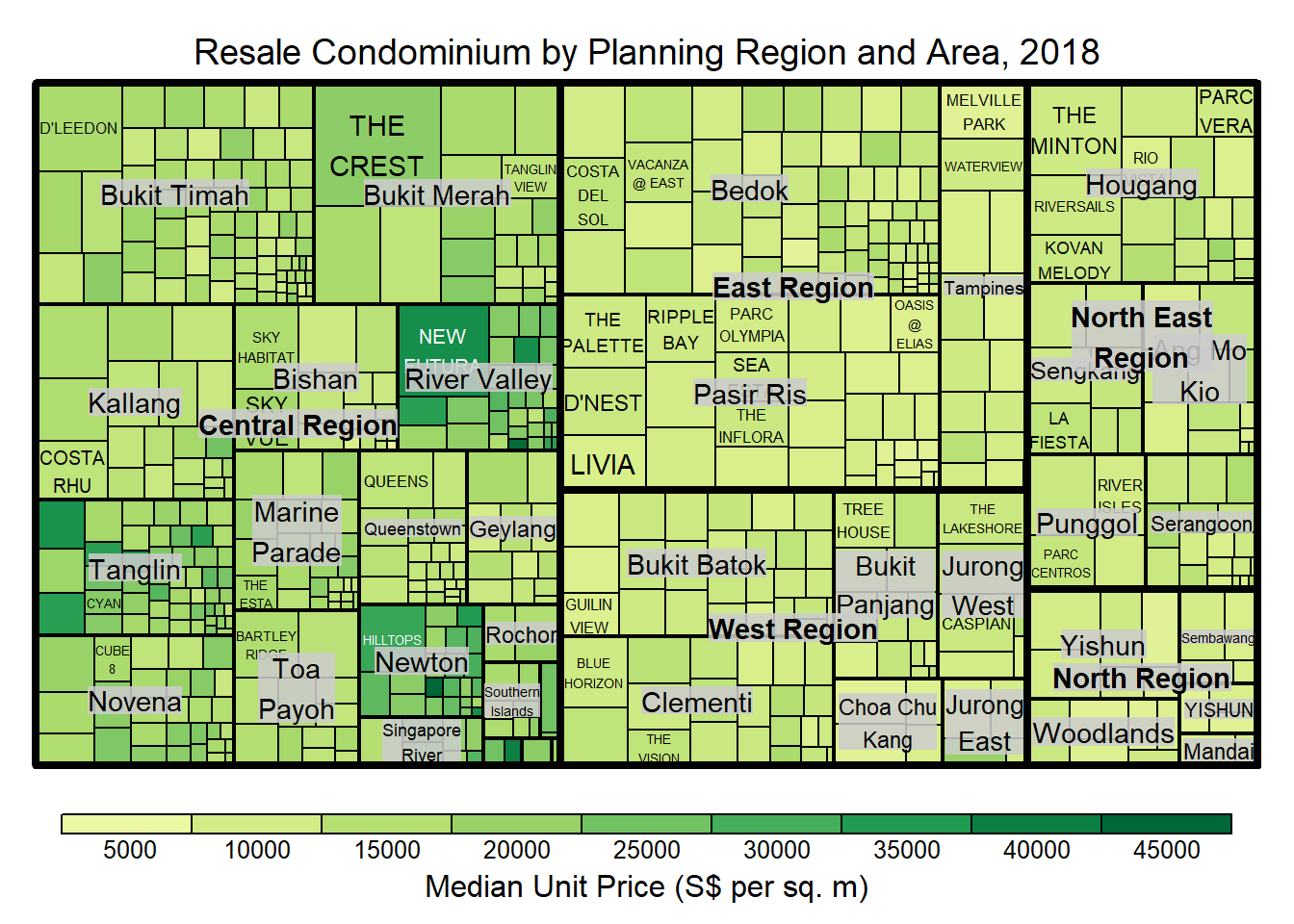
Note
The rectangles are coloured with different intensities of green, reflecting their respective median unit prices.
The legend reveals that the values are binned into ten bins, i.e. 0-5000, 5000-10000, etc. with an equal interval of 5000.
Two arguments that determine the mapping to colour palettes: mapping and palette. We will focus on palette here.
If type = “value”, treemap considers palette to be a diverging color palette (say ColorBrewer’s “RdYlBu”), and maps it in such a way that 0 corresponds to the middle color (typically white or yellow), -max(abs(values)) to the left-end color, and max(abs(values)), to the right-end color.
If type = “manual”, treemap simply maps min(values) to the left-end color, max(values) to the right-end color, and mean(range(values)) to the middle color.
Show the code
treemap(realis2018_selected,
        index=c("Planning Region", "Planning Area", "Project Name"),
        vSize="Total Unit Sold",
        vColor="Median Unit Price ($ psm)",
        type="value",
        palette="RdYlBu",
        title="Resale Condominium by Planning Region and Area, 2018",
        title.legend = "Median Unit Price (S$ per sq. m)" )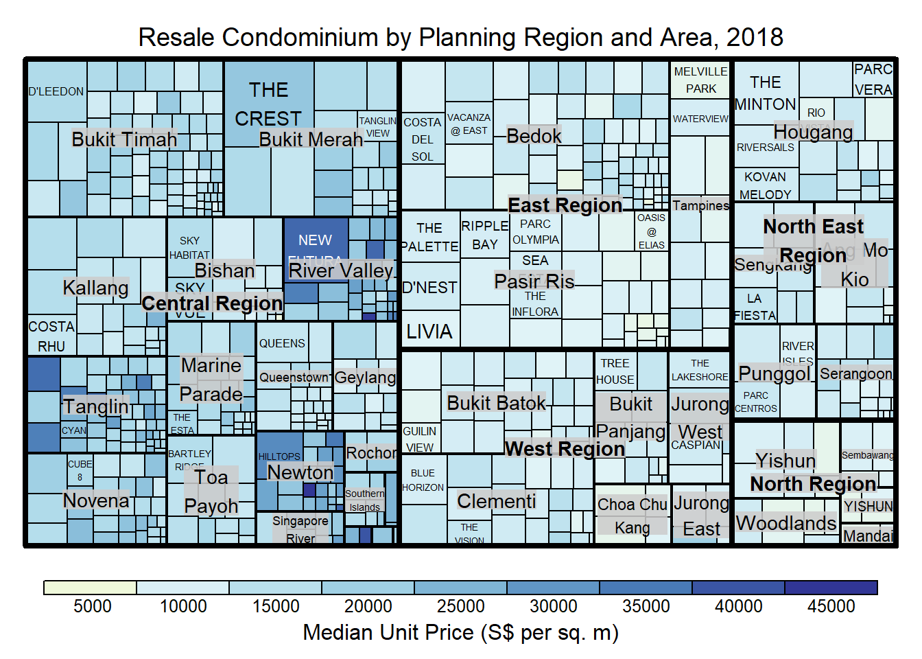
Note
Although the colour palette used is ‘RdYlBu’ but there are no red rectangles in the treemap above. This is because all the median unit prices are positive. The reason why we see only 5000 to 45000 in the legend is because the range argument is by default c(min(values, max(values)) with some pretty rounding.
Show the code
treemap(realis2018_selected,
        index=c("Planning Region", "Planning Area", "Project Name"),
        vSize="Total Unit Sold",
        vColor="Median Unit Price ($ psm)",
        type="manual",
        palette="Blues",
        title="Resale Condominium by Planning Region and Area, 2018",
        title.legend = "Median Unit Price (S$ per sq. m)" )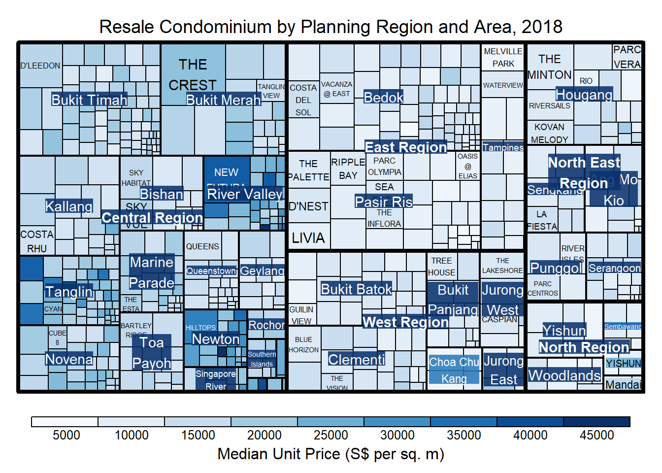
Tip
It is not wise to use diverging colour palette such as ‘RdYlBu’ if the values are all positive or negative. Choose a single colour like ‘Blues’
treemap() supports two popular treemap layouts, namely: “squarified” and “pivotSize”. The default is “pivotSize”.
The squarified treemap algorithm (Bruls et al., 2000) produces good aspect ratios, but ignores the sorting order of the rectangles (sortID). The ordered treemap, pivot-by-size, algorithm (Bederson et al., 2002) takes the sorting order (sortID) into account while aspect ratios are still acceptable.
Show the code
treemap(realis2018_selected,
        index=c("Planning Region", "Planning Area", "Project Name"),
        vSize="Total Unit Sold",
        vColor="Median Unit Price ($ psm)",
        type="manual",
        palette="Blues",
        algorithm = "squarified",
        title="Resale Condominium by Planning Region and Area, 2018",
        title.legend = "Median Unit Price (S$ per sq. m)")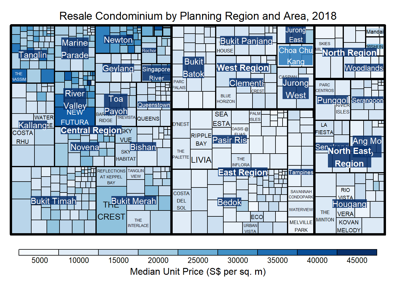
When “pivotSize” algorithm is used, sortID argument can be used to determine the order in which the rectangles are placed from top left to bottom right.
Show the code
treemap(realis2018_selected,
        index=c("Planning Region", "Planning Area", "Project Name"),
        vSize="Total Unit Sold",
        vColor="Median Unit Price ($ psm)",
        type="manual",
        palette="Blues",
        algorithm = "pivotSize",
        sortID = "Median Transacted Price",
        title="Resale Condominium by Planning Region and Area, 2018",
        title.legend = "Median Unit Price (S$ per sq. m)" )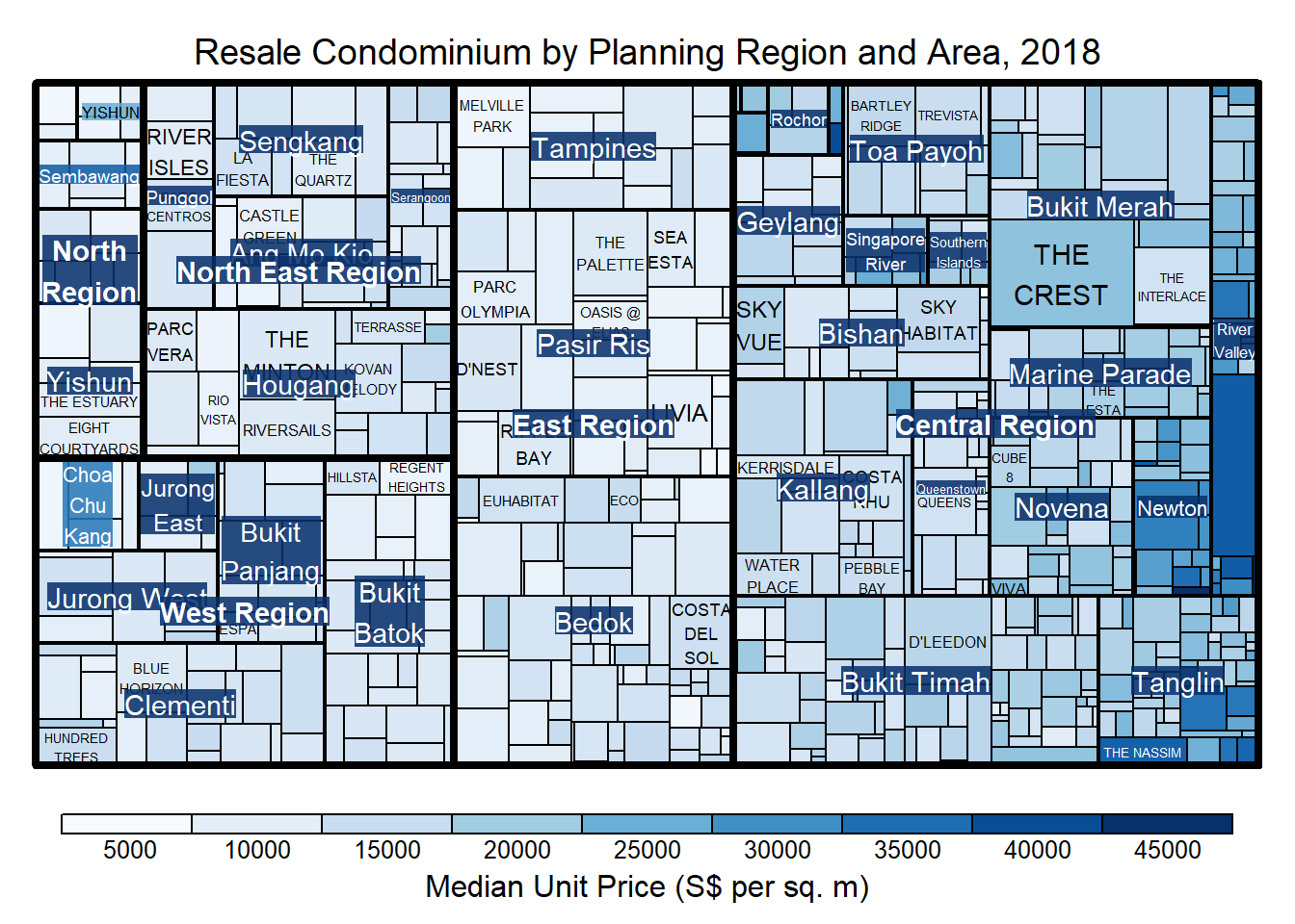
4 Designing Static Treemap using treemapify Package
treemapify is a R package specially developed to draw treemaps in ggplot2.
More information on Introduction to “treemapify” and its user guide.
Show the code
ggplot(data=realis2018_selected,
       aes(area = `Total Unit Sold`,
           fill = `Median Unit Price ($ psm)`),
       layout = "scol",
       start = "bottomleft") +
  geom_treemap() +
  scale_fill_gradient(low = "light blue", high = "blue")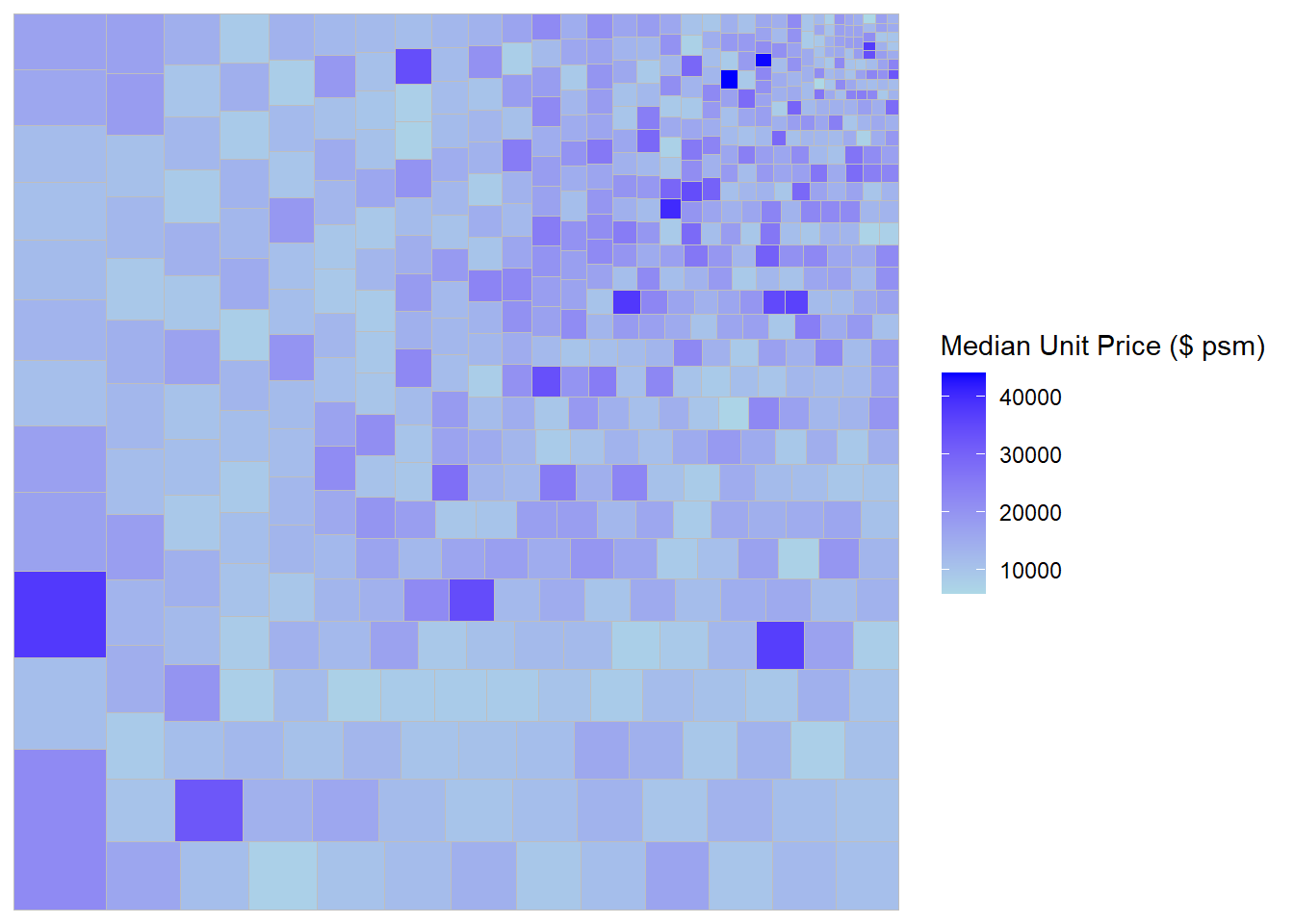
There are several ways to group to define hierachy.
Show the code
ggplot(data=realis2018_selected,
       aes(area = `Total Unit Sold`,
           fill = `Median Unit Price ($ psm)`,
           subgroup = `Planning Region`),
       start = "topleft") +
  geom_treemap()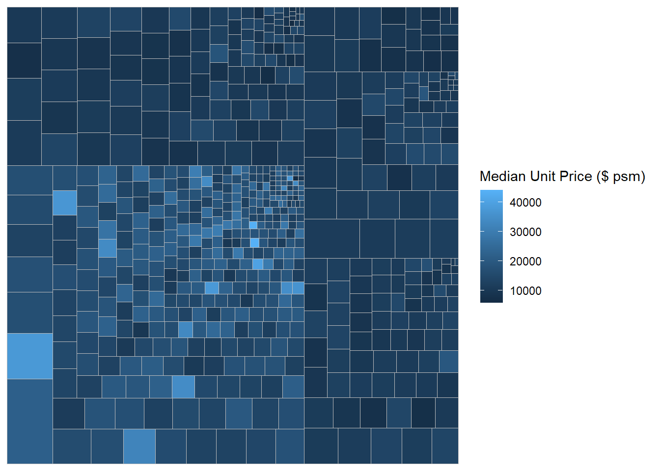
Show the code
ggplot(data=realis2018_selected,
       aes(area = `Total Unit Sold`,
           fill = `Median Unit Price ($ psm)`,
           subgroup = `Planning Region`,
           subgroup2 = `Planning Area`)) +
  geom_treemap()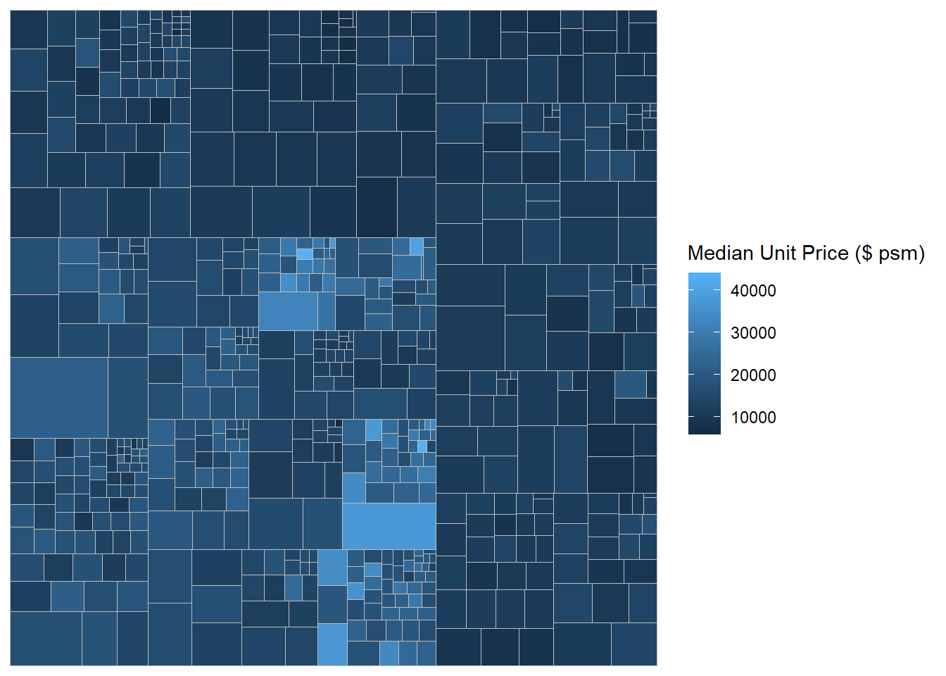
Show the code
ggplot(data=realis2018_selected,
       aes(area = `Total Unit Sold`,
           fill = `Median Unit Price ($ psm)`,
           subgroup = `Planning Region`,
           subgroup2 = `Planning Area`)) +
  geom_treemap() +
  geom_treemap_subgroup2_border(colour = "gray40",
                                size = 2) +
  geom_treemap_subgroup_border(colour = "gray20")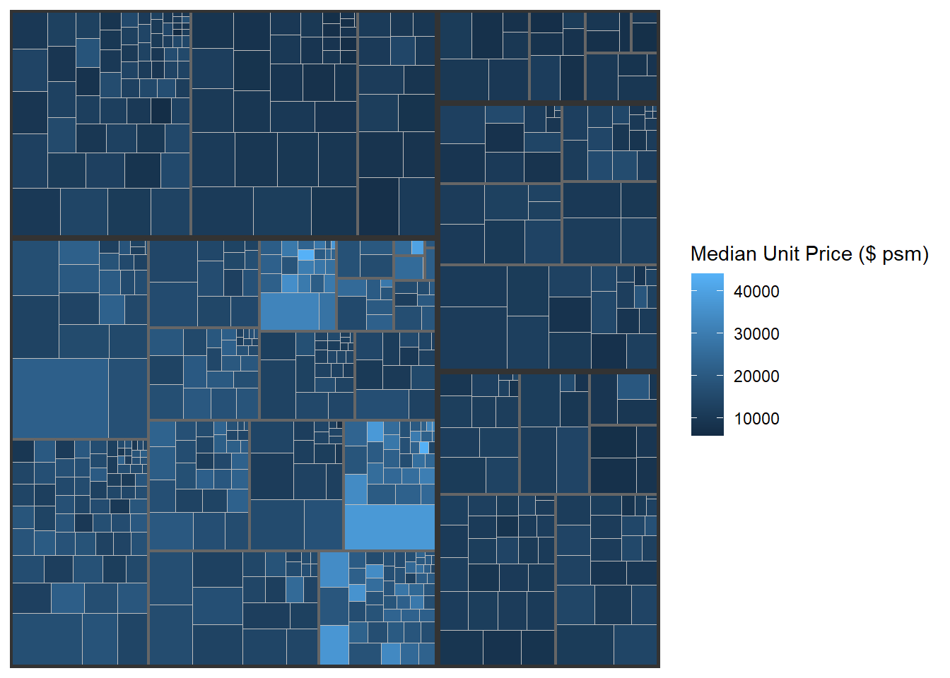
5 Designing Interactive Treemaps using d3treeR
Two steps to create an interactive treemap.
Create a treemap by using selected variables in condominium data frame.
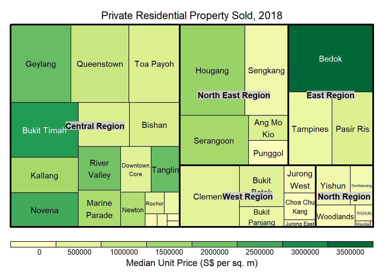
Show the code
tm <- treemap(realis2018_summarised,
        index=c("Planning Region", "Planning Area"),
        vSize="Total Unit Sold",
        vColor="Median Unit Price ($ psm)",
        type="value",
        title="Private Residential Property Sold, 2018",
        title.legend = "Median Unit Price (S$ per sq. m)" )
Use d3tree to build the interactive treemap.
Show the code
tm2 <- treemap(realis2018_summarised,
        index=c("Planning Region", "Planning Area"),
        vSize="Total Unit Sold",
        vColor="Median Unit Price ($ psm)",
        type="value",
        title="Private Residential Property Sold, 2018",
        title.legend = "Median Unit Price (S$ per sq. m)"
        )
d3tree(tm2, rootname = "Singapore" )